How to Use the VLOOKUP Function in Excel

If Excel had a hall of fame, VLOOKUP would already have a plaque, a retirement speech, and probably a fan club made up of accountants, analysts, office managers, and anyone who has ever tried to match one spreadsheet with another without losing their mind. The function may look a little intimidating at first, but once you understand its logic, it becomes one of the handiest tools in your spreadsheet toolbox.

At its core, the VLOOKUP function in Excel helps you search for a value in the first column of a table and return a related value from another column in the same row. In plain American English, it is the digital version of saying, “Find this ID, then tell me the department, price, status, or whatever else is sitting beside it.”

In this guide, you’ll learn exactly how to use VLOOKUP, when to choose an exact match versus an approximate match, how to troubleshoot common errors, and why this formula still matters even in a world where XLOOKUP is trying to steal the spotlight. We’ll also walk through practical examples so the whole thing feels less like abstract spreadsheet wizardry and more like something you can actually use today.

What Is VLOOKUP in Excel?

VLOOKUP stands for vertical lookup. The “vertical” part matters because the function searches down the first column of a selected range. Once Excel finds the item you asked for, it pulls back a value from another column in that same row.

Let’s say you have an employee list with IDs in column A, names in column B, and departments in column C. If you know the employee ID and want the department, VLOOKUP can do that in seconds. Instead of manually scanning row after row like you’re hunting for a missing sock, Excel does the work for you.

This makes VLOOKUP useful for tasks like matching product IDs to prices, finding customer names from account numbers, pulling inventory details from a master sheet, checking commission rates, or combining data from two spreadsheets that share a common identifier.

VLOOKUP Syntax Explained

The basic formula looks like this:

Here’s what each argument means:

1. lookup_value

This is the value you want Excel to search for. It can be a cell reference like A2, a number, or text in quotation marks.

2. table_array

This is the range where Excel should search. The lookup value must be in the first column of this range. That rule is not flexible. Excel did not come here to negotiate.

3. col_index_num

This is the column number inside your selected range that contains the value you want returned. If your table array is F2:H10, then column F is 1, G is 2, and H is 3.

4. range_lookup

This tells Excel whether you want an exact match or an approximate match.

• FALSE means exact match.
• TRUE means approximate match.

Most of the time, especially for names, IDs, email addresses, invoice numbers, and product codes, you’ll want FALSE.

How to Use the VLOOKUP Function in Excel: 8 Simple Steps

Step 1: Organize Your Data

Before you write a single formula, make sure the value you want to look up appears in the leftmost column of your lookup range. If your product ID is in column C and the price is in column A, VLOOKUP will not be happy. It only looks to the right.

Step 2: Identify the Value You Want to Find

Pick the unique value you’ll use as your match key. This might be a customer ID, SKU, employee number, or order code. Unique identifiers work best because duplicates can return the first matching result, which may or may not be the one you wanted.

Step 3: Select the Table Array

Choose the full data range that contains both the lookup column and the return column. If your data runs from F2:H10, that entire range becomes your table array.

Step 4: Lock the Range with Absolute References

If you plan to copy the formula down a column, use dollar signs so the table array stays fixed:

Without absolute references, the range may shift as you drag the formula downward, which is Excel’s way of turning a simple task into an avoidable mystery.

Step 5: Count the Return Column Correctly

Count from the left side of your selected range, not from column A of the worksheet. If your table array is F2:H10 and the return value is in column H, the correct col_index_num is 3.

Step 6: Choose Exact or Approximate Match

Use FALSE when you need an exact result. Use TRUE only when your first column is sorted in ascending order and you want the closest match below or equal to the lookup value, such as tax brackets, grading scales, or commission tiers.

Step 7: Enter the Formula

Here’s a simple exact-match example:

This formula looks for the value in A2 in the first column of F2:H10 and returns the value from the third column of that range.

Step 8: Copy It Down and Check Results

Once the first formula works, drag it down to fill the rest of the column. Then spot-check a few rows. Never trust a spreadsheet just because it looks confident.

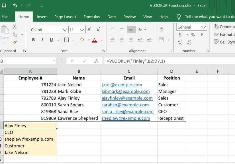
VLOOKUP Exact Match Example

Imagine you have this setup:

• Column A: Product ID
• Column F: Product ID in a master table
• Column G: Product Name
• Column H: Price

You want Excel to return the price for the product ID in A2. Use:

Why this works:

• A2 is the lookup value.
• $F$2:$H$100 is the table array.
• 3 returns the price from the third column in that range.
• FALSE demands an exact match.

This is the most common way people use the Excel VLOOKUP formula, especially when merging information from a master reference table into a working report.

VLOOKUP Approximate Match Example

Approximate match is useful when values fall into ranges rather than needing perfect one-to-one matches. Think grades, commission percentages, shipping rates, or tax brackets.

Suppose you have a score in B2 and a grading scale in columns J and K:

If B2 contains 87, Excel will look for the largest value less than or equal to 87 in the first column of the table and return the grade tied to that threshold.

One huge warning: the first column in an approximate-match table must be sorted in ascending order. If it is not sorted, Excel can return the wrong result, and it will do so with the calm confidence of someone giving bad directions at a gas station.

How to Use VLOOKUP Across Two Sheets

One of the best uses for VLOOKUP is pulling information from another worksheet. Let’s say your current sheet contains order IDs, and another sheet named Prices contains the matching product prices.

In this example:

• A2 is the order or product code you want to match.
• Prices! tells Excel to search in the sheet named Prices.
• $A$2:$C$200 is the lookup table on that sheet.
• 3 returns the value from the third column.
• FALSE requires an exact match.

This kind of VLOOKUP between two spreadsheets or two sheets is incredibly useful when cleaning data, building sales reports, or joining exported lists from different systems.

Common VLOOKUP Errors and How to Fix Them

#N/A Error

This usually means Excel can’t find a match. Common causes include:

• The value doesn’t exist in the first column of the table array
• You used FALSE and there is no exact match
• The data contains extra spaces or hidden characters
• Numbers are stored as text

To make results look cleaner, wrap the formula in IFERROR:

#REF! Error

This appears when your col_index_num is larger than the number of columns in the table array. If your range has only three columns and you ask for column 4, Excel throws a small but justified tantrum.

Wrong Value Returned

This often happens when:

• You forgot to set FALSE for exact matching
• Your approximate-match table is not sorted
• Your lookup range shifted because you didn’t lock it with dollar signs
• The lookup column contains duplicates

Text and Number Formatting Problems

If one column stores IDs as text and the other stores them as numbers, VLOOKUP may not match them. Also check for leading or trailing spaces. Functions like TRIM and CLEAN can help tidy messy data before you run the lookup.

Helpful VLOOKUP Tips That Save Time

Use Exact Match by Default

For most business, school, and reporting tasks, exact match is safer. If you’re matching IDs, email addresses, invoice numbers, or employee records, stick with FALSE.

Use Wildcards for Partial Matches

If you’re working with text and need a partial match, VLOOKUP can use wildcard characters when the last argument is FALSE.

This can match values that begin with “Ander”. A question mark ? matches a single character, and an asterisk * matches a sequence of characters.

Know the Left-to-Right Limitation

VLOOKUP can only return values from columns to the right of the lookup column. If you need to look left, consider INDEX and MATCH or, in newer versions of Excel, XLOOKUP.

Be Careful with Inserted Columns

Because VLOOKUP relies on a numeric column index, inserting or rearranging columns can break your logic or return the wrong field. That is one reason some Excel users move to XLOOKUP once it becomes available to them.

VLOOKUP vs. XLOOKUP: Which One Should You Use?

VLOOKUP is still useful, widely recognized, and found in many existing workbooks. But in newer versions of Excel, XLOOKUP is the more flexible option.

XLOOKUP can search in any direction, uses separate lookup and return arrays, and returns an exact match by default. It also tends to be easier to read once you get used to it. That said, VLOOKUP remains worth learning because plenty of businesses still use older files packed with it like canned soup in a storm pantry.

If you’re just starting out, learn VLOOKUP first so you understand the lookup logic. Then learn XLOOKUP so future-you can work faster and complain less.

Real-World Example You Can Copy

Here’s a practical setup for pulling employee departments based on employee ID:

Assume:

• A2 contains the employee ID you want to check
• Column M contains employee IDs
• Column N contains department names
• Column O contains office locations

If you want the office location instead of the department, change the third argument from 2 to 3:

Once you understand that one small change, you unlock a whole lot of spreadsheet power.

Experience: What Using VLOOKUP Actually Feels Like in Real Life

Learning VLOOKUP is one thing. Using it in the wild is another. And by “the wild,” I mean the slightly chaotic world of shared spreadsheets, mystery exports, renamed columns, and that one file your coworker made in 2018 that still runs half the department.

For many people, the first real VLOOKUP moment happens when two spreadsheets need to become friends. Maybe one file has customer IDs and order dates, while another holds names, cities, and account status. You could copy and paste manually, of course, but that path usually leads to errors, eye strain, and an afternoon that feels five business days long. VLOOKUP steps in like a practical hero. It matches the shared ID and brings the missing information over with minimal drama, assuming the data is clean and Excel is in a cooperative mood.

One of the most common experiences with VLOOKUP is the sudden appearance of #N/A in places where you were emotionally expecting success. At first, that error feels rude. Later, you learn it is actually useful. It tells you something is off. Maybe the lookup value has an extra space. Maybe one sheet stores numbers as text. Maybe someone typed “00125” in one file and “125” in another. VLOOKUP becomes less of a formula and more of a detective partner, pointing at where your data hygiene needs work.

Another real-world lesson is that exact match usually saves the day. New users sometimes leave the last argument blank, not realizing Excel defaults to approximate match. That can produce results that look valid but are quietly wrong, which is the most dangerous kind of wrong. Once you experience that once, you become the person who always types FALSE with the confidence of a seasoned Excel veteran.

Then there is the absolute-reference lesson. Nearly everyone writes a perfectly good VLOOKUP formula, drags it down, and watches it break because the table array moved. After that, the dollar sign stops looking weird and starts looking like a loyal friend. The same goes for checking whether the lookup column is actually on the left. VLOOKUP has rules, and it rewards people who respect them.

In daily work, VLOOKUP is especially satisfying when you use it to clean up imported data, match HR records, connect sales reports, fill in missing product information, or verify prices from a master table. It turns repetitive tasks into fast ones. It also makes you look like the person who “knows Excel,” which is both flattering and a great way to inherit more spreadsheet problems.

Over time, VLOOKUP teaches a bigger lesson than syntax. It teaches structure. Good spreadsheet work depends on clean identifiers, consistent formatting, logical tables, and careful checking. In that sense, VLOOKUP is not just a formula. It is a tiny management seminar hiding inside a cell.

Conclusion

If you want to work faster in Excel, understanding how to use the VLOOKUP function in Excel is a smart move. It helps you search vertically through a table, pull matching data from another column, combine information across sheets, and reduce hours of manual copy-and-paste. The key is remembering the fundamentals: your lookup value must be in the first column of the selected range, your column index number is counted within that range, and FALSE is usually the safest choice for exact matches.

Once you get comfortable with the formula, VLOOKUP stops feeling technical and starts feeling practical. It becomes one of those Excel skills you’ll reuse again and again, whether you’re organizing a budget, cleaning a report, comparing datasets, or rescuing a project from spreadsheet chaos.